Modified Mori-Tanaka Scheme

import numpy as np
import matplotlib.pyplot as plt
plt.rcParams['font.size']=14
plt.rcParams['font.family']='arial'

import rockphypy # import the module
from rockphypy import EM

Modified Mori-Tanaka scheme

Iwakuma (et al.) proposed a modified Mori-Tanaka scheme in which the fraction of matrix is set to zero, for simplicity, only spherical inhomogeneities are considered, the two phase composite with a virtual martix is

\[\bar{K}=\frac{ {\textstyle \sum_{i=1}^{2}} \frac{f_iK_i}{1-(1-\frac{K_i}{K_M} ) \alpha } }{{\textstyle \sum_{i=1}^{2}} \frac{f_i}{1-(1-\frac{K_i}{K_M} ) \alpha } }\]

\[\bar{G}=\frac{ {\textstyle \sum_{i=1}^{2}} \frac{f_iG_i}{1-(1-\frac{G_i}{G_M} ) \alpha } }{{\textstyle \sum_{i=1}^{2}} \frac{f_i}{1-(1-\frac{G_i}{G_M} ) \alpha } }\]

\[f_1+f_2=1\]

Note that the material parameters of the matrix which no longer exists still remain in these expressions and has great impact on the result

Relationship between Modifiedl MT scheme and Hashin strikmann bound

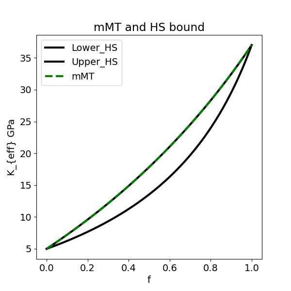
If the virtual matrix is set equivalent to one of the inhomogeneities, for example, if we set \(K_m\) to \(K_1\) and \(\nu_M= \nu_1\), then the mMT becomes one of the Hashin–Shtrikman bounds. The derivation is shown as follows:

\[\bar{K}=\frac{f_1K_1+\frac{f_2K_2}{1-(1-\frac{K_2}{K_1} )\alpha } }{f_1+\frac{f_2}{1-(1-\frac{K_2}{K_1} )\alpha }}\]

\[\frac{\bar{K}}{K_1} =\frac{f_1+\frac{f_2\frac{K_2}{K_1} }{1-(1-\frac{K_2}{K_1} )\alpha } }{f_1+\frac{f_2}{1-(1-\frac{K_2}{K_1} )\alpha }}\]

\[\frac{\bar{K}}{K_1} =\frac{f_1-f_1(1-\frac{K_2}{K_1} )\alpha +f_2\frac{K_2}{K_1} }{f_1-f_1(1-\frac{K_2}{K_1} )\alpha +f_2}\]

\[\frac{\bar{K}}{K_1} =\frac{f_1+f_2-f_1(1-\frac{K_2}{K_1} )\alpha +f_2\frac{K_2}{K_1}-f_2 }{f_1-f_1(1-\frac{K_2}{K_1} )\alpha +f_2}\]

\[\frac{\bar{K}}{K_1} =\frac{1-f_1(1-\frac{K_2}{K_1} )\alpha +f_2(\frac{K_2}{K_1}-1) }{1-f_1(1-\frac{K_2}{K_1} )\alpha }\]

\[\frac{\bar{K}}{K_1} =1+\frac{f_2(\frac{K_2}{K_1}-1) }{1-f_1(1-\frac{K_2}{K_1} )\alpha }\]

\[\frac{\bar{K}}{K_1} =1-\frac{f_2(1-\frac{K_2}{K_1}) }{1-f_1(1-\frac{K_2}{K_1} )\alpha }\]

Next we show modified MT scheme is upper Hashin-Shtrikmann bound.

\(\alpha\) is one of the coefficient of Elsheby Tensor defined as a function of Poisson’s ratio of the virtual matrix \(\nu_M=\frac{3K-2G}{2(3K+G)}\)

\[\alpha \equiv \frac{1+\nu_M}{3(1-\nu_M)}\]

The Hashin-Strikmann bound is:

\[K^{HS}=K_1+\frac{f_2}{(K_2-K_1)^{-1}+f_1(K_1+\frac{4}{3}G_1 )^{-1}}\]

\[\alpha = \frac{3K}{3K+4G}\]

Let’s denote \(\frac{K_2}{K_1}-1\) as \(M\),

\[\frac{\bar{K}}{K_1} =1+\frac{f_2 }{\frac{1}{M}+f_1\alpha }\]

\[\frac{\bar{K}}{K_1} =1+\frac{f_2 }{\frac{K_1}{K_2-K_1} +f_1\alpha }\]

\[\bar{K}=K_1+\frac{f_2K_1\cdot \frac{1}{K_1} }{ (\frac{K_1}{K_2-K_1} +f_1\alpha)\cdot \frac{1}{K_1} }\]

\[\bar{K} = K_1+\frac{f_2}{ \frac{1}{K_2-K_1} +f_1\frac{ \alpha}{K_1} }\]

\[\bar{K} = K_1+\frac{f_2}{ (K_2-K_1)^{-1} +f_1\frac{ \alpha}{K_1} }\]

\[\bar{K} = K_1+\frac{f_2}{ (K_2-K_1)^{-1} +f_1 (K_1+\frac{4}{3}G_1 )^{-1} }\]

Example

Let’s see if the modified mori-Tanaka scheme will yield the same result as given by HS upper bound when set the virtual matrix constant to be the phase 1’s constant, phase 1 is stiff, and phase 2 is soft

f= np.linspace(0,1,100)
Ki, Gi=5,10 #
Km, Gm=37,45  #  65, 30

# model
K_UHS, GUHS= EM.HS(f, Km, Ki,Gm, Gi, bound='upper')
K_LHS, GLHS= EM.HS(f, Km, Ki,Gm, Gi, bound='lower')
K_MT, G_MT= EM.MT_average(f, Km, Gm,Km, Gm, Ki, Gi)

fig=plt.figure(figsize=(6,6))
plt.xlabel('f')
plt.ylabel('K_{eff} GPa')
#plt.xlim(0,20)
#plt.ylim(2.5,5.5)
plt.title('mMT and HS bound')
plt.plot(f,K_LHS,'-k',lw=3,label='Lower_HS')
plt.plot(f,K_UHS,'-k',lw=3,label='Upper_HS')
plt.plot(f,K_MT,'g--',lw=3,label='mMT')
plt.legend(loc='upper left')
#plt.text(0, 190, 'K1/G1=K2/G2=50 \n\\nu=0.3')

<matplotlib.legend.Legend object at 0x7f70f2496550>

Reference Iwakuma, T. and Koyama, S., 2005. An estimate of average elastic moduli of composites and polycrystals. Mechanics of materials, 37(4), pp.459-472.