Elastic bounds

This example shows the comparison between different elastic bounds to Nur’s cirtical porosity model: Voigt and Reuss Bounds, Voigt–Reuss–Hill Average,Hashin-Shtrikmann bounds

import numpy as np
import matplotlib.pyplot as plt
plt.rcParams['font.size']=14
plt.rcParams['font.family']='arial'

import rockphypy # import the module for rock physics
from rockphypy import EM # import the "effective medium" EM module
# import the 'Fluid' module
from rockphypy import Fluid

Voigt and Reuss Bounds

At any given volume fraction of constituents, the effective modulus will fall between the bounds. In the lecture we learn that the Voigt upper bound \(M_v\) of N phases are defined as:

\[M_V=\sum_{i=1}^{N}f_iM_i\]

The Reuss lower bound is

\[\frac{1}{M_R} =\sum_{i=1}^{N}\frac{f_i}{M_i}\]

where \(f_i\) is the volume fraction of the ith phase and \(M_i\) is the elastic bulk or shear modulus of the ith phase.

Voigt–Reuss–Hill Average Moduli Estimate

This average is simply the arithmetic average of the Voigt upper

bound and the Reuss lower bound.

\[M_{VRH}=\frac{M_V+M_R}{2}\]

bell:

For fluid-solid composite, calculation of Reuss, Voigt and VRH bounds are straightforward. Here we give a generalized function to compute effective moduli of N-phases composite:

Hashin-Shtrikmann bounds

The Voigt and Reuss bounds are simply arithmetic and harmonic averages. The Hashin-Shtrikman bounds are stricter than the Reuss-Voigt bounds. The two-phase HS bounds can be written as:

\[K^{\mathrm{HS} \pm}=K_{1}+\frac{f_{2}}{\left(K_{2}-K_{1}\right)^{-1}+f_{1}\left(K_{1}+\frac{4}{3} \mu_{1}\right)^{-1}}\]

\[\mu^{\mathrm{HS} \pm}=\mu_{1}+\frac{f_{2}}{\left(\mu_{2}-\mu_{1}\right)^{-1}+2 f_{1}\left(K_{1}+2 \mu_{1}\right) /\left[5 \mu_{1}\left(K_{1}+\frac{4}{3} \mu_{1}\right)\right]}\]

where the superscript +/− indicates upper or lower bound respectively. \(K_1\) and \(K_2\) are the bulk moduli of individual phases; \(\mu_1\) and \(\mu_2\) are the shear moduli of individual phases; and \(f_1\) and \(f_2\) are the volume fractions of individual phases. The upper and lower bounds are computed by interchanging which material is termed 1 and which is termed 2. The expressions yield the upper bound when the stiffest material is termed 1 and the lower bound when the softest material is termed 1. The expressions shown in the lectures represents the HS bound for fluid-solid composite.

Examples

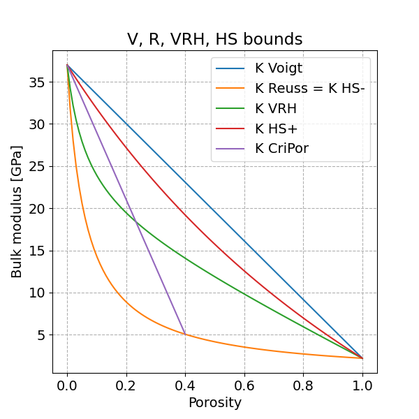
Let’s compute effective bulk and shear moduli of a water saturated rock using different bound models.

Here we also make a comparision with Nur’s critical porosity model as introduced in the previous example.

# specify model parameters
phi=np.linspace(0,1,100,endpoint=True) # solid volume fraction = 1-phi
K0, G0= 37,44 # moduli of grain material
Kw, Gw= 2.2,0 # moduli of water
# VRH bounds
volumes= np.vstack((1-phi,phi)).T
M= np.array([K0,Kw])
K_v,K_r,K_h=EM.VRH(volumes,M)
# Hashin-Strikmann bound
K_UHS,G_UHS= EM.HS(1-phi, K0, Kw,G0,Gw, bound='upper')
# Critical porosity model
phic=0.4 # Critical porosity
phi_=np.linspace(0.001,phic,100,endpoint=True) # solid volume fraction = 1-phi
K_dry, G_dry= EM.cripor(K0, G0, phi_, phic)# Compute dry-rock moduli
Ksat, Gsat = Fluid.Gassmann(K_dry,G_dry,K0,Kw,phi_)# saturate rock with water

# plot
plt.figure(figsize=(6,6))
plt.xlabel('Porosity')
plt.ylabel('Bulk modulus [GPa]')
plt.title('V, R, VRH, HS bounds')
plt.plot(phi, K_v,label='K Voigt')
plt.plot(phi, K_r,label='K Reuss = K HS-')
plt.plot(phi, K_h,label='K VRH')
plt.plot(phi, K_UHS,label='K HS+')
plt.plot(phi_, Ksat,label='K CriPor')
plt.legend(loc='best')
plt.grid(ls='--')

Reference: Mavko, G., Mukerji, T. and Dvorkin, J., 2020. The rock physics handbook. Cambridge university press.