Self Consistent (SC) Estimation

import numpy as np
import matplotlib.pyplot as plt
plt.rcParams['font.size']=14
plt.rcParams['font.family']='arial'

import rockphypy # import the module
from rockphypy import EM

Dilute distribution of spherical inclusion without self consistency

the coefficients of Eshelby tensor S1 and S2 are functions of the matrix Poisson’s ratio

\[\nu_M=\frac{3K-2G}{2(3K+G)}\]

\[S_1=\frac{1+\nu}{3(1-\nu)}\]

\[S_2=\frac{2(4-5\nu)}{15(1-\nu)}\]

As a special case, let all micro-inclusions have the same elasticity, with the common bulk and shear moduli \(K_i\), If the macrostress is regarded prescribed, then

\[\frac{\bar{K}}{K_m}=\left \{ {1+f(\frac{K_m}{K_m-K_i}-S_1 )^{-1}} \right \} ^{-1}\]

\[\frac{\bar{G}}{G_m}=\left \{ {1+f(\frac{G_m}{G_m-G_i}-S_2 )^{-1}} \right \} ^{-1}\]

and and if the macrostrain is regarded prescribed:

\[\frac{\bar{K}}{K_m}= {1-f(\frac{K_m}{K_m-K_i}-S_1 )^{-1}}\]

\[\frac{\bar{G}}{G_m}= {1-f(\frac{G_m}{G_m-G_i}-S_2 )^{-1}}\]

Self consistent estimates

If the distribution of micro-inclusions is random and the interaction effects are to be included to a certain extent, then the self-consistent method may be used to estimate the overall response of the RVE. Now \(S_1\) and \(S_2\) are defined in terms of the overall Poisson ratio

\[\bar{\nu}\equiv \frac{3\bar{K} -2\bar{G}}{2(3\bar{K}+\bar{G})}\]

\[\bar{S_1}=\frac{1+\bar{\nu}}{3(1-\bar{\nu})}\]

\[\bar{S_2}=\frac{2(4-5\bar{\nu})}{15(1-\bar{\nu})}\]

When all micro-inclusions consist of the same material, denote their common bulk and shear moduli by \(K_i\), then

\[\frac{\bar{K}}{K_m}=1-\frac{\bar{K}(K_m-K_i) }{K_m(\bar{K}-K_i )}(\frac{\bar{K} }{\bar{K}-K_i}-\bar{S_1} )^{-1}\]

\[\frac{\bar{G}}{G_m}=1-\frac{\bar{G}(G_m-G_i) }{G_m(\bar{G}-G_i )}(\frac{\bar{G} }{\bar{G}-G_i}-\bar{S_2} )^{-1}\]

It is noted that although \(\bar{K}\) and \(\bar{G}\) given by dilute distribution estimates are decoupled, by self consistent estimates are coupled, so iterative solver is invoked in SC approach.

Example

Let’s compare the Dilute distribution/ Non interacting estimates to the SC estimation for spherical inclusion. The overall bulk and shear moduli of the media with randomly distributed spherical inclusion sastifies Ki/Km= Gi/Gm=50, \(\nu_i=\nu_m=\frac{1}{3}\)

#  Specify model parameters
ro=13/6
Km, Gm=3*ro, 3 #
Ki, Gi=Km*50, Gm*50  #  65, 30
f= np.linspace(0,0.4,100)
iter_n= 100
#  Dilute distribution of inclusion without self consistency
K_stress, G_stress= EM.SC_dilute(Km, Gm, Ki, Gi, f, 'stress')
K_strain, G_strain= EM.SC_dilute(Km, Gm, Ki, Gi, f, 'strain')

#   Self Consistent estimates
Keff,Geff= EM.SC_flex(f,iter_n,Km,Ki,Gm,Gi)

# plot
fig=plt.figure(figsize=(6,6))
plt.xlabel('f')
plt.ylabel('K_{eff} GPa')
plt.xlim(0,0.4)
plt.ylim(0,4)
plt.title('self_consistent model comparision')

plt.plot(f,K_stress,'-k',lw=2,label='Macrostress prescribed')
plt.plot(f,K_strain,'--k',lw=2,label='Macrostrain prescribed')
plt.plot(f,Keff/Km,'-r',label='SC')

plt.legend(loc='best')
fig=plt.figure(figsize=(6,6))
plt.ylim(0,4)
plt.xlim(0,0.4)
plt.xlabel('f')
plt.ylabel('G_{eff} GPa')
plt.plot(f,G_stress,'-k',lw=2,label='Macrostress prescribed')
plt.plot(f,G_strain,'--k',lw=2,label='Macrostrain prescribed')
plt.plot(f,Geff/Gm,'-r',label='SC')
plt.legend(loc='best')

• 
• 

<matplotlib.legend.Legend object at 0x000002132B69B100>

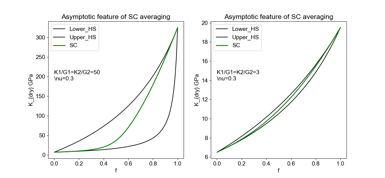
Let’s compare the SC model with Hashin-strikmann bound, It’s anticipated that the SC model will show asymptotic features

# Comparision with HS bounds

# large difference of material parameters
f= np.linspace(1e-3,0.9999,100)
ro=13/6
Ki, Gi=3*ro, 3 #
Km, Gm=Ki*50, Gi*50  #  65, 30
iter_n= 1000
# model
K_UHS, GUHS= EM.HS(f, Km, Ki,Gm, Gi, bound='upper')
K_LHS, GLHS= EM.HS(f, Km, Ki,Gm, Gi, bound='lower')
K_SC, G_SC= EM.SC_flex(f,iter_n,Ki,Km,Gi,Gm)

#fig=plt.figure(figsize=(6,6))
plt.figure(figsize=(13,6))
plt.subplot(121)
plt.xlabel('f')
plt.ylabel('K_{dry} GPa')
#plt.xlim(0,20)
#plt.ylim(2.5,5.5)
plt.title('Asymptotic feature of SC averaging')
plt.plot(f,K_LHS,'-k',label='Lower_HS')
plt.plot(f,K_UHS,'-k',label='Upper_HS')
plt.plot(f,K_SC,'g-',lw=2,label='SC')
plt.legend(loc='upper left')
plt.text(0, 190, 'K1/G1=K2/G2=50 \n\\nu=0.3')

# small difference of material parameters
ro=13/6
Ki, Gi=3*ro, 3 #
Km, Gm=Ki*3, Gi*3
K_UHS, GUHS= EM.HS(f, Km, Ki,Gm, Gi, bound='upper')
K_LHS, GLHS= EM.HS(f, Km, Ki,Gm, Gi, bound='lower')
K_SC, G_SC= EM.SC_flex(f,iter_n,Ki,Km,Gi,Gm)
plt.subplot(122)
plt.xlabel('f')
plt.ylabel('K_{dry} GPa')
#plt.xlim(0,20)
#plt.ylim(2.5,5.5)
plt.title('Asymptotic feature of SC averaging')
plt.plot(f,K_LHS,'-k',label='Lower_HS')
plt.plot(f,K_UHS,'-k',label='Upper_HS')
plt.plot(f,K_SC,'g-',lw=2,label='SC')
plt.legend(loc='upper left')
plt.text(0,14, 'K1/G1=K2/G2=3 \n\\nu=0.3')

Text(0, 14, 'K1/G1=K2/G2=3 \n\\nu=0.3')

Reference: - Nemat-Nasser, S. and Hori, M., 2013. Micromechanics: overall properties of heterogeneous materials. Elsevier. - Iwakuma, T. and Koyama, S., 2005. An estimate of average elastic moduli of composites and polycrystals. Mechanics of materials, 37(4), pp.459-472.