Note
Go to the end to download the full example code
Patchy cement model
import numpy as np
import matplotlib.pyplot as plt
plt.rcParams['font.size']=14
plt.rcParams['font.family']='arial'
plt.rcParams['axes.labelpad'] = 10.0
#plt.rcParams["font.weight"] = "bold"
# import the module
from rockphypy import EM, GM
Patchy cement model (PCM) is proposed by Avseth (2016) and mainly applied to high porosity cemented clean sandstone. Patchy means the sandstone is weakly to intermediately cemented. The microstructure of the represented as an effective medium comprising a mixture of two end member: cemented sandstones (where all grain contacts are cemented) and loose, unconsolidated sands. The cemented sandstone can be modeled using the Dvorkin-Nur model, whereas the loose sand end member can be modeled using the Hertz-Mindlin (or Walton) contact theory. The effective dry-rock moduli for a patchy cemented high-porosity end member then can be formulated as follows:
Assuming stiff isotropic mixture according to the Hashin-Shtrikman upper bound,
Assuming soft isotropic mixture according to the Hashin-Shtrikman lower bound
where \(K_{cem}\) and \(K_{unc}\) are the dry-rock bulk moduli of cemented rock and unconsolidated rock, respectively; \(\mu_{cem}\) and \(\mu_{unc}\) are the ditto dry-rock shear moduli; and \(f\) is the volume fraction of cemented rock in the binary mixture of cemented and unconsolidated rock of the patchy cemented rock.
The GM.pcm is the implementation of the patchy cement model provided by rockphypy.
Example
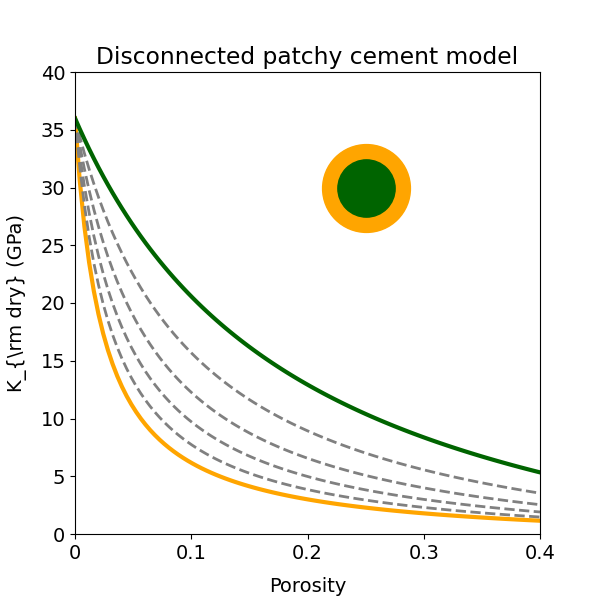
Rock-physics modeling of patchy cemented sandstone, for which the connected patchy cement and disconnected patchy cement are modeled.
# specify model parameters
Dqz, Kqz, Gqz = 2.65, 36, 42 ## grain density, bulk and shear modulus
Dsh, Ksh, Gsh = 2.7, 21, 7 # shale/clay density, bulk and shear modulus
Dc,Kc, Gc =2.65, 36, 42 # cement density, bulk and shear modulus
vsh=0

_,_,K0=EM.VRH(np.array([vsh,1-vsh]),np.array([Ksh,Kqz])) # clay fraction can be considered.
_,_,G0=EM.VRH(np.array([vsh,1-vsh]),np.array([Gsh,Gqz]))

phic=0.4 # critical porosity
f=np.linspace(0,1,6) # volume fraction of the stiff phase in the binary mixture.
sigma=10
phi=np.linspace(1e-6,phic,100)
Cn=6
v_cem=0.1
v_ci=0.111
scheme=2
f_=0 #reduce shear factor
fig=plt.figure(figsize=(6,6))
plt.xlabel('Porosity',labelpad=10)
plt.ylabel(r'K_{\rm dry} (GPa)',labelpad=10)
plt.xlim(0,0.4)
plt.xticks([0, 0.1, 0.2, 0.3,0.4], ['0', '0.1', '0.2', '0.3','0.4'])
#plt.yticks([0, 10, 20, 30,40], ['0', '1', '2', '3','4'])
plt.ylim(0,40)
#plt.title('Connected patchy cement')
for i,val in enumerate(f):
    if val==0:
        kwargs  =   {'color':"orange", # for edge color
             'linewidth':3, # line width of spot
             'linestyle':'-', # line style of spot
            }
    elif val==1:
        kwargs  =   {'color':"darkgreen", # for edge color
             'linewidth':3, # line width of spot
             'linestyle':'-', # line style of spot
            }
    else:
        kwargs  =   {'color':"grey", # for edge color
             'linewidth':2, # line width of spot
             'linestyle':'--', # line style of spot
            }
    Kdry,Gdry=GM.pcm(val,sigma, K0,G0,phi, phic,v_cem,v_ci, Kc,Gc,Cn=Cn, mode='stiff',scheme=scheme,f_=f_)

    plt.plot(phi,Kdry,**kwargs)
plt.scatter(0.25,30,s=4000, c='darkgreen')
plt.scatter(0.25,30,s=1700, c='orange')
plt.title('Connected patchy cement model')

Text(0.5, 1.0, 'Connected patchy cement model')
fig=plt.figure(figsize=(6,6))
plt.xlabel('Porosity',labelpad=10)
plt.ylabel(r'K_{\rm dry} (GPa)',labelpad=10)
plt.xlim(0,0.4)
plt.xticks([0, 0.1, 0.2, 0.3,0.4], ['0', '0.1', '0.2', '0.3','0.4'])
plt.ylim(0,40)
#plt.title('Disconnected patchy cement')
for i,val in enumerate(f):
    if val==0:
        kwargs  =   {'color':"orange", # for edge color
             'linewidth':3, # line width of spot
             'linestyle':'-', # line style of spot
            }
    elif val==1:
        kwargs  =   {'color':"darkgreen", # for edge color
             'linewidth':3, # line width of spot
             'linestyle':'-', # line style of spot
            }
    else:
        kwargs  =   {'color':"grey", # for edge color0
             'linewidth':2, # line width of spot
             'linestyle':'--', # line style of spot
            }
    Kdry,Gdry=GM.pcm(val,sigma, K0,G0,phi,  phic,v_cem,v_ci, Kc,Gc,Cn=Cn,mode='soft',scheme=scheme,f_=f_)
    plt.plot(phi,Kdry,**kwargs)
# plot HS coating relation animation
plt.scatter(0.25,30,s=4000, c='orange')
plt.scatter(0.25,30,s=1700, c='darkgreen')
plt.title('Disconnected patchy cement model')
Text(0.5, 1.0, 'Disconnected patchy cement model')
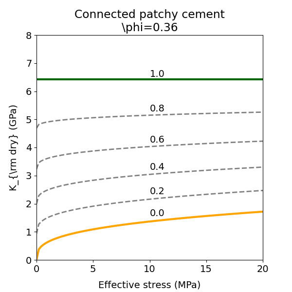
Estimate stress sensitivity of sandstone using PCM
By varing the effective stress at given porosity, the stress sensitivities of patchy cement sandstone can be modeled.
sigma=np.linspace(1e-7,20,100) # varing effective stress
phi=0.36 # fix porosity

fig=plt.figure(figsize=(6,6))
plt.xlabel('Effective stress (MPa)')
plt.ylabel(r'K_{\rm dry} (GPa)')
plt.xticks([0, 5, 10, 15,20], ['0', '5', '10', '15','20'])
#xticks([0,5,10,15,20])
#ax1.set_xticklabels(['0', '5','10','15','20'])
plt.xlim(0,20)
plt.ylim(0,8)
#plt.subplot(121)
plt.title('Connected patchy cement\n\phi=0.36')

for i,val in enumerate(f):
    if val==0:
        kwargs  =   {'color':"orange", # for edge color
             'linewidth':3, # line width of spot
             'linestyle':'-', # line style of spot
            }
    elif val==1:
        kwargs  =   {'color':"darkgreen", # for edge color
             'linewidth':3, # line width of spot
             'linestyle':'-', # line style of spot
            }
    # elif val==0.8:
    #     kwargs  =   {'color':"red", # for edge color
    #          'linewidth':3, # line width of spot
    #          'linestyle':'--', # line style of spot
    #         }
    else:
        kwargs  =   {'color':"grey", # for edge color
             'linewidth':2, # line width of spot
             'linestyle':'--', # line style of spot
            }
    Kdry,Gdry=GM.pcm(val,sigma, K0,G0,phi,  phic,v_cem,v_ci, Kc,Gc,Cn=Cn,mode='stiff',scheme=scheme,f_=f_)
    plt.plot(sigma,Kdry,**kwargs)
    plt.text(10,Kdry[60]+0.1,'{:.1f}'.format(val))
fig=plt.figure(figsize=(6,6))
plt.xlabel('Effective stress (MPa)')
plt.ylabel(r'K_{\rm dry} (GPa)')
plt.xticks([0, 5, 10, 15,20], ['0', '5', '10', '15','20'])

plt.xlim(0,20)
plt.ylim(0,8)
plt.title('Disconnected patchy cement\n\phi=0.36')

for i,val in enumerate(f):
    if val==0:
        kwargs  =   {'color':"orange", # for edge color
             'linewidth':3, # line width of spot
             'linestyle':'-', # line style of spot
            }
    elif val==1:
        kwargs  =   {'color':"darkgreen", # for edge color
             'linewidth':3, # line width of spot
             'linestyle':'-', # line style of spot
            }
    # elif val==0.8:
    #     kwargs  =   {'color':"darkblue", # for edge color
    #          'linewidth':3, # line width of spot
    #          'linestyle':'--', # line style of spot
    #         }
    else:
        kwargs  =   {'color':"grey", # for edge color
             'linewidth':2, # line width of spot
             'linestyle':'--', # line style of spot
            }
    Kdry,Gdry=GM.pcm(val,sigma, K0,G0,phi,  phic,v_cem,v_ci, Kc,Gc,Cn=Cn,mode='soft',scheme=scheme,f_=f_)
    plt.plot(sigma,Kdry,**kwargs)
    plt.text(10,Kdry[60]+0.06,'{:.1f}'.format(val))

Reference
Avseth, P., Skjei, N. and Mavko, G., 2016. Rock-physics modeling of stress sensitivity and 4D time shifts in patchy cemented sandstones—Application to the Visund Field, North Sea. The Leading Edge, 35(10), pp.868-878.
Yu, J., Duffaut, K., and Avseth, P. 2023, Stress sensitivity of elastic moduli in high-porosity-cemented sandstone — Heuristic models and experimental data, Geophysics, 88(4)
Total running time of the script: (0 minutes 0.630 seconds)
