Rock Physics Template (RPT)

import pandas as pd
import numpy as np
import matplotlib.pyplot as plt
plt.rcParams['font.size']=14
plt.rcParams['font.family']='arial'

#import rockphypy # import the module
from rockphypy import QI, GM, Fluid

Rock physics models can be used to calculate elastic properties with various combination of lithology and fluid parameters. Rock Physics Templates (RPTs) were first presented by Ødegaard and Avseth (2003). Rock physics templates (RPT) is used to display a reference framework of all the possible variations of a particular rock and use such templates to understand actual well log data (or seismic-derived elastic properties).

# specify model parameters
D0, K0, G0 = 2.65, 36.6, 45
Dc,  Kc, Gc = 2.65,37, 45 # cement
Db, Kb = 1, 2.5
Do, Ko = 0.8, 1.5
Dg, Kg = 0.2, 0.05
### adjustable para
phi_c = 0.4
Cn=8.6  ## calculate coordination number
phi = np.linspace(0.1,phi_c,10) #define porosity range according to critical porosity
sw=np.linspace(0,1,5) # water saturation
sigma=20
f=0.5

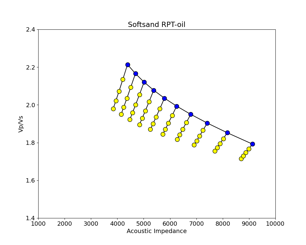
• Case 1: create RPT for unconsolidated sand using softsand/friable sand model

# softsand model gas
Kdry1, Gdry1 = GM.softsand(K0, G0, phi, phi_c, Cn, sigma,f) # soft sand
fig1=QI.plot_rpt(Kdry1,Gdry1,K0,D0,Kb,Db,Kg,Dg,phi,sw)
plt.title('Softsand RPT-gas')
plt.xlim(1000,10000)
plt.ylim(1.4,2.4)

(1.4, 2.4)

# softsand model oil
fig1_=QI.plot_rpt(Kdry1,Gdry1,K0,D0,Kb,Db,Ko,Do,phi,sw)
plt.title('Softsand RPT-oil')
plt.xlim(1000,10000)
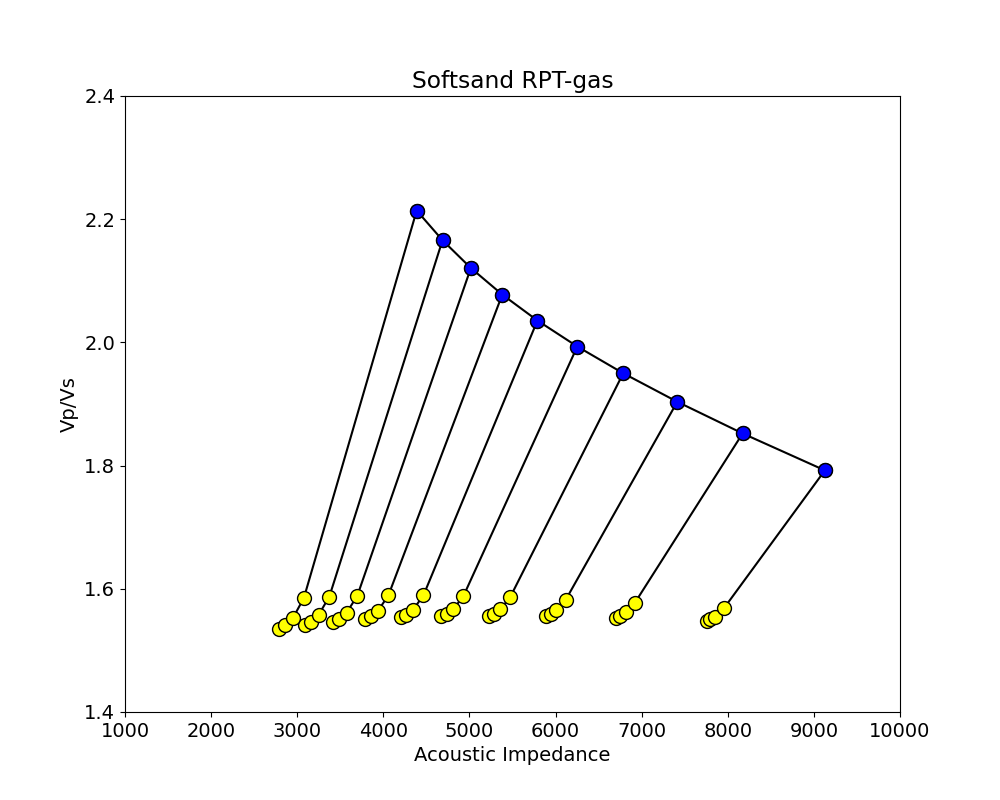
plt.ylim(1.4,2.4)

(1.4, 2.4)

• Case 2: create RPT for stiff sandstone using stiffsand model

Kdry2, Gdry2 = GM.stiffsand(K0, G0, phi, phi_c, Cn, sigma, f) # stiff sand
fig2=QI.plot_rpt(Kdry2,Gdry2,K0,D0,Kb,Db,Kg,Dg,phi,sw)
plt.title('Stiffsand RPT-gas')
plt.xlim(1000,14000)
plt.ylim(1.4,2.3)

(1.4, 2.3)

# stiffsand model oil
fig2_=QI.plot_rpt(Kdry2,Gdry2,K0,D0,Kb,Db,Ko,Do,phi,sw)
plt.title('Stiffsand RPT-oil')
plt.xlim(1000,14000)
plt.ylim(1.4,2.3)

(1.4, 2.3)

Applied to field data

Let’s import the same synthetic well log data and apply the rock physics screening to the well log data

# read data
data = pd.read_csv('../../data/well/sandstone.csv',index_col=0)
# specify model parameters
D0, K0, G0 = 2.65, 37, 38
Dg, Kg = 0.2, 0.05
### adjustable para
phi_c = 0.36
phi = np.linspace(0.01,phi_c,10) #define porosity range according to critical porosity
sw=np.linspace(0,1,5) # water saturation
IP= data.VP*data.DEN
PS= data.VP/data.VS
Kdry, Gdry = GM.stiffsand(K0, G0, phi, phi_c, Cn, sigma, f=0) # stiff sand

# sphinx figure
# sphinx_gallery_thumbnail_number = 5
fig=QI.plot_rpt(Kdry,Gdry,K0,D0,Kb,Db,Kg,Dg,phi,sw)
fig.set_size_inches(7, 6)
plt.scatter(IP,PS, c=data.eff_stress,edgecolors='grey',s=80,alpha=1,cmap='Greens_r')
cbar=plt.colorbar()
cbar.set_label(r'$\rm \sigma_{eff}$ (MPa)')
plt.xlabel('IP')
plt.xlim(1000,14000)
plt.ylim(1.4,2.4)
#fig.savefig(path+'./rpt.png',dpi=600,bbox_inches='tight')

(1.4, 2.4)

Reference:

• Mavko, G., Mukerji, T. and Dvorkin, J., 2020. The rock physics handbook. Cambridge university press.

• Avseth, P.A. and Odegaard, E., 2003. Well log and seismic data analysis using rock physics templates. First break, 22(10).

• Avseth, P., Mukerji, T. and Mavko, G., 2010. Quantitative seismic interpretation: Applying rock physics tools to reduce interpretation risk. Cambridge university press.