CO2 seismic properties

A interesting question about \(CO_2\) injection is how to estimate the seismic properties of the \(CO_2\)-water mixture. This notebook shows how to perform Gassmann fluid substitution of a sandstone injected with \(CO_2\).

We want to solve the following questions through modelling:

1. Velocity drop resulted from \(CO_2\) displacing brine in an unconsolidated sand

2. How different would it be if it is \(CO_2\) in gas phase compared to supercritical \(CO_2\).

3. How to model the impact of saturation. i.e. difference between patchy saturation or uniform saturation.

The modelling process is as follows:

The initial unconsolidated sand is brine saturated. The dry rock properties are modeled using Hertz-Mindlin (HM) with porosity = 0.4, coordination number = 6 at 15 MPa.

The gas \(CO_2\) is modeled at temperature = 17 degree and pressure 5 Mpa, The critical \(CO_2\) is modeled at temperature = 60 degree and 10 Mpa.

The gas saturation varies from 0 to 100%, uniform and patchy saturation are concerned.

Though the above modelling is quite simplified, we can learn how to use building blocks, i.e. functions of rockphypy to solve pratical questions.

from rockphypy import utils, BW, GM, Fluid
import numpy as np
import matplotlib.pyplot as plt
import pandas as pd

plt.rcParams['font.size'] = 14
plt.rcParams['font.family'] = 'arial'

plt.rcParams["figure.figsize"] = (6, 6)
plt.rcParams['axes.labelpad'] = 10.0


# grain and brine para
D0, K0, G0 = 2.65, 36, 42  # grain density, bulk and shear modulus
Db, Kb = 1, 2.2  # brine density, bulk modulus

# reservoir condition and brine salinity
P_overburden = 20  # Mpa
salinity = 35000/1000000
# HM
phi_c = 0.4  # critical porosity
Cn = 6  # coordination number

• initial state: 100% water saturation at specific temperature and pressure, the reservoir stress condition is predefined with a given overburden pressure 20Mpa.

• Case 1: uniform gasesous \(CO_2\) mixed with brine.

# saturation condition
brie = None
temperature = 17
pore_pressure = 5  # pore pressure
sigma = P_overburden-pore_pressure  # effective stress
# softsand model to compute the frame properties
Kdry, Gdry = GM.softsand(K0, G0, phi_c, phi_c, Cn, sigma, f=0.5)  # soft sand
# C02 in gas condition:
sw = np.linspace(0, 1, 50)  # water saturation
sco2 = 1-sw
# gaseous co2 mixed with brine, temp=17, pore pressure = 5Mpa
den1, Kf_mix_1 = BW.co2_brine(temperature, pore_pressure,
                           salinity, sco2, brie_component=brie)
vp1, vs1, rho1 = Fluid.vels(Kdry, Gdry, K0, D0, Kf_mix_1, den1, phi_c)

• Case 2: uniform critical \(CO_2\) mixed with brine.

# C02 in critical condition: the critical condition of c02 is 31.1° C, 7.4Mpa.

brie = None
temperature = 60
pore_pressure = 10  # pore pressure
sigma = P_overburden-pore_pressure  # effective stress
# softsand model to compute the frame properties
Kdry, Gdry = GM.softsand(K0, G0, phi_c, phi_c, Cn, sigma, f=0.5)  # soft sand
# C02 in critical condition:
den2, Kf_mix_2 = BW.co2_brine(temperature, pore_pressure, salinity,
                           sco2, brie_component=brie)  # gas co2 mixed with brine
vp2, vs2, rho2 = Fluid.vels(Kdry, Gdry, K0, D0, Kf_mix_2, den2, phi_c)

plt.figure()
name = 'Uniform saturation'
plt.title(name)
plt.plot(sco2, vp1/1000, '-k', label='Gas CO2')
plt.plot(sco2, vp2/1000, '-r', label='Critical CO2')
plt.xlabel('CO2 saturation')
plt.grid(ls='--')
plt.ylabel('Vp (Km)')
plt.legend(loc='best')

<matplotlib.legend.Legend object at 0x7f70f24966a0>

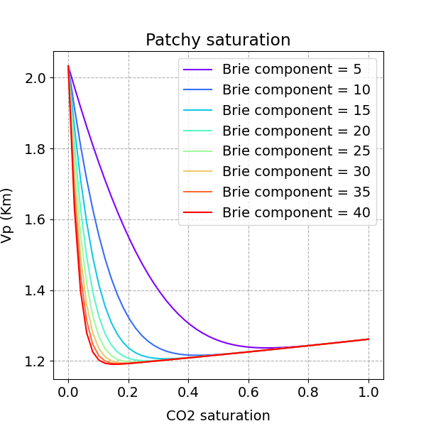
• Case 3: patchy saturated critical \(CO_2\) mixed with brine.

# sphinx_gallery_thumbnail_number = 2
brie = np.arange(5, 45, 5)
colors = plt.cm.rainbow(np.linspace(0, 1, len(brie)))
plt.figure()
name = 'Patchy saturation'
plt.title(name)
plt.xlabel('CO2 saturation')
plt.grid(ls='--')
plt.ylabel('Vp (Km)')


for i, val in enumerate(brie):
    den, Kf_mix = BW.co2_brine(temperature, pore_pressure, salinity,
                            sco2, brie_component=val)  # gas co2 mixed with brine
    vp, vs, rho = Fluid.vels(Kdry, Gdry, K0, D0, Kf_mix, den, phi_c)

    plt.plot(sco2, vp/1000, c=colors[i],
             label='Brie component = {}'.format(val))

plt.legend(loc='best')

<matplotlib.legend.Legend object at 0x7f70f23d1dc0>

Reference

• Xu, H. (2006). Calculation of CO2 acoustic properties using Batzle-Wang equations. Geophysics, 71(2), F21-F23.