Note
Go to the end to download the full example code
Improved CO2 properties modelling using Batzle-Wang
Using the Batzle-Wang equations for gas to calculate CO2 properties is a common in seismic modelling. Nonetheless, this method can result in substantial inaccuracies, particularly when dealing with elevated fluid pressure.
from rockphypy import utils, BW, GM, Fluid
import numpy as np
import matplotlib.pyplot as plt
import pandas as pd

plt.rcParams['font.size'] = 14
plt.rcParams['font.family'] = 'arial'

plt.rcParams["figure.figsize"] = (6, 6)
plt.rcParams['axes.labelpad'] = 10.0
First we write a function that computes the the effective properties of \(CO_2\)-brine mixture given different saturation, temperature, pressure and salinity of the brine. The \(CO_2\) property as a function of temperature and pressure is modeled using the modified version of Batzle-Wang proposed by Xu 2006, see the documentation of BW.rho_K_co2. The critical \(CO_2\) property is better modeled using Xu’s approach.
This method has been included in BW class, it can be called via BW.co2_brine
def co2_brine(temperature, pressure, salinity, Sco2, brie_component=None, bw=False):
    """compute the effective properties of critical Co2 brine mixture depending on temperature, pressure and salinity of the brine, as well as the saturation state.

    Args:
        temperature (degree)
        pressure (Mpa): pore pressure, not effective stress
        salinity (ppm): The weight fraction of NaCl, e.g. 35e-3
            for 35 parts per thousand, or 3.5% (the salinity of
            seawater).
        Sco2 (frac): Co2 saturation
        brie_component (num): if None: uniform saturation. otherwise patchy saturation according to brie mixing

    Returns:
        den_mix (g/cc): mixture density
        Kf_mix (GPa): bulk modulus
    """
    G = 1.5349
    if bw is True:
        rho_co2, K_co2 = BW.rho_K_gas(pressure, temperature, G)
    else:
        rho_co2, K_co2 = BW.rho_K_co2(pressure, temperature, G)

    rho_brine, K_b = BW.rho_K_brine(temperature, pressure, salinity)

    den_mix = (1-Sco2)*rho_brine+Sco2*rho_co2

    if brie_component == None:
        Kf_mix = ((1-Sco2)/K_b+Sco2/K_co2)**-1  # Woods formula

    else:
        # patchy saturation
        Kf_mix = Fluid.Brie(K_b, K_co2, 1-Sco2, brie_component)
    # print('Kco2',K_co2,'K_b', K_b)
    # print('density',den_mix,'moduli',Kf_mix)
    return den_mix, Kf_mix
comparison between original BW and modified BW for CO2 properties at temperature = 57 degree.
temp = 57  # temperature
G = 1.5349  # gas gravity of CO2
p = np.linspace(0, 60, 100)  # pore pressure
rho_co2, K_co2 = BW.rho_K_co2(p, temp, G)  # new BW prediction
rho_co2_BW, K_co2_BW = BW.rho_K_gas(p, temp, G)  # original BW prediction

# import the data of co2 properties measured by wang and nur
path = '../../data'
K_data = pd.read_csv(path+'/wang_K.csv')
den_data = pd.read_csv(path+'/wang_den.csv')
den_data = den_data.sort_values(by='pressure')

fig1 = plt.figure(figsize=(4, 4))
plt.plot(p, K_co2, '-k', lw=3, label='BW_new')
plt.plot(p, K_co2_BW, '-.k', label='BW')
plt.ylim(0, 1.4)
plt.xlim(0, 40)
plt.plot(K_data.pressure, K_data.K, '--', c='r', label='Lab data')
plt.xlabel('Pressure (MPa)')
plt.ylabel('K (GPa)')
plt.legend()
# fig1.savefig(path+'/figure1.png',dpi=600,bbox_inches='tight')
fig2 = plt.figure(figsize=(4, 4))

plt.plot(p, rho_co2, '-k', lw=3, label='BW_new')
plt.plot(p, rho_co2_BW, '-.k', label='BW')
plt.plot(den_data.pressure, den_data.density, '--', c='r')
plt.ylim(0, 1)
plt.xlim(0, 40)
plt.xlabel('Pressure (MPa)')
plt.ylabel(r'Density (g/${\rm cm^3}$)')
# fig2.savefig(path+'/figure2.png',dpi=600,bbox_inches='tight')

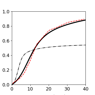
Text(-4.486111111111111, 0.5, 'Density (g/${\\rm cm^3}$)')
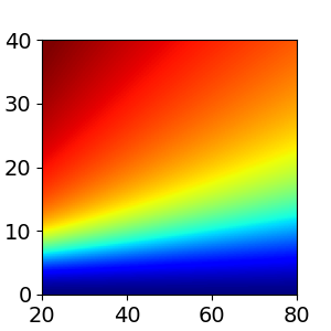
Bulk modulus (top rows) and density (bottom rows) of pure CO2 as a function of pressure and temperature. 2D plot
pressure = np.linspace(0, 40, 100)
temperature = np.linspace(20, 80, 100)
P, T = np.meshgrid(pressure, temperature, indexing='ij')

rho_co2, K_co2 = BW.rho_K_co2(P, T, G)  # K in Mpa
rho_co2_BW, K_co2_BW = BW.rho_K_gas(P, T, G)  # original BW prediction

extent = np.min(temperature), np.max(
    temperature), np.min(pressure), np.max(pressure)


# sphinx_gallery_thumbnail_number = 3
fig = plt.figure(figsize=(3, 3))


im = plt.imshow(rho_co2, aspect=6/4, origin='lower', cmap='jet', extent=extent)
plt.xlabel('Temperature (°C)')
plt.ylabel('Pressure (MPa)')
# plt.title('Density B-W new',pad=10, fontsize=16)
cb_ax = fig.add_axes([1.05, 0, .05, 1])
cbar = fig.colorbar(im, orientation='vertical', cax=cb_ax)
plt.clim(0, 1)
# cbar=plt.colorbar(im)
cbar.set_label(r'Density (g/${\rm cm^3}$)', size=16, labelpad=10)
######### difference caused by BW #######################
# grain and brine para
D0, K0, G0 = 2.65, 36, 42  # grain density, bulk and shear modulus
Db, Kb = 1, 2.2  # brine density, bulk modulus

# reservoir condition and brine salinity
P_overburden = 20  # Mpa
salinity = 35000/1000000

# HM
phi_c = 0.4  # critical porosity
Cn = 6  # coordination number

overburden_stress = 40
pore_pressure = 20
sigma = overburden_stress-pore_pressure  # effective stress
# saturation condition
brie = 4
temperature = 45

# softsand model to compute the frame properties
Kdry, Gdry = GM.softsand(K0, G0, phi_c, phi_c, Cn, sigma, f=1)  # soft sand
# C02 in gas condition:
sw = np.linspace(0, 1, 50)  # water saturation
sco2 = 1-sw

# compute the CO2 properties using original BW
# gaseous co2 mixed with brine, temp=17, pore pressure = 5Mpa
den1, Kf_mix_1 = co2_brine(temperature, pore_pressure,
                           salinity, sco2, brie_component=brie, bw=True)
vp1, vs1, rho1 = Fluid.vels(Kdry, Gdry, K0, D0, Kf_mix_1, den1, phi_c)
compute the CO2 properties using modified BW gaseous co2 mixed with brine, temp=17, pore pressure = 5Mpa
fig = plt.figure(figsize=(5, 4))

plt.plot(sco2, vp1/1000, '-.k', lw=3, label='B-W')
plt.plot(sco2, vp2/1000, '-r', lw=3, label='B-W New')
plt.plot(sco2, vs1/1000, '-.k',lw=3)
plt.plot(sco2, vs2/1000,'--r', lw=3)

plt.xlabel(r' ${\rm S_{CO_2}}$')
plt.grid(ls='--')
plt.ylabel('Velocity (Km/s)')
plt.legend(loc='best')
plt.ylim(0.8, 2.4)
plt.xlim(0, 1)
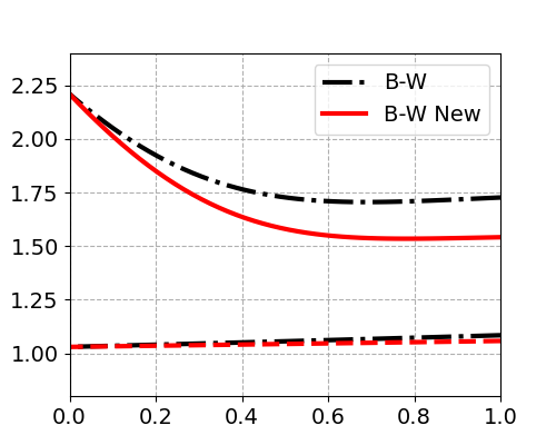
(0.0, 1.0)
Reference
Xu, H. (2006). Calculation of CO2 acoustic properties using Batzle-Wang equations. Geophysics, 71(2), F21-F23.
Total running time of the script: (0 minutes 0.614 seconds)
